Closed Loop Transfer Function Matlab
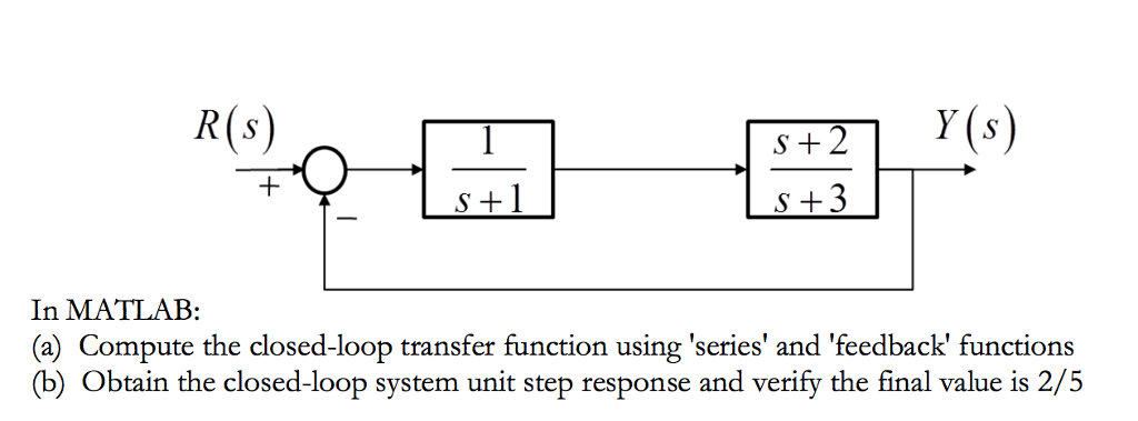
Solved In Matlab A Compute The Closed Loop Transfer Fun Chegg Com
Control Tutorials For Matlab And Simulink Extras Steady State Error
Using Feedback To Close Feedback Loops Matlab Simulink Example

Closed Loop Transfer Function From Generalized Model Of Control System Matlab Getiotransfer Mathworks Italia

Find Closed Loop Transfer Function From The Open Loop Transfer Function For A Unity Feedback
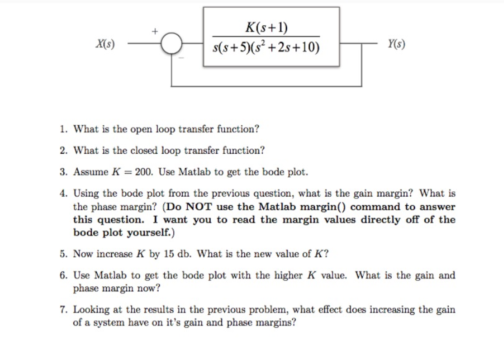
Solved What Is The Open Loop Transfer Function What Is T Chegg Com
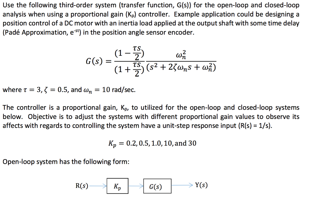
Modeling of dc motor in matlab more detail.
Closed loop transfer function matlab.
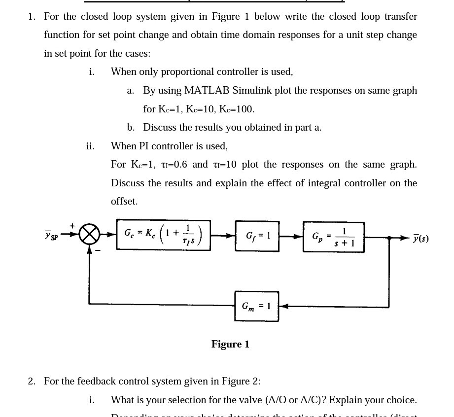
1 For The Closed Loop System Given In Figure 1 Be Chegg Com
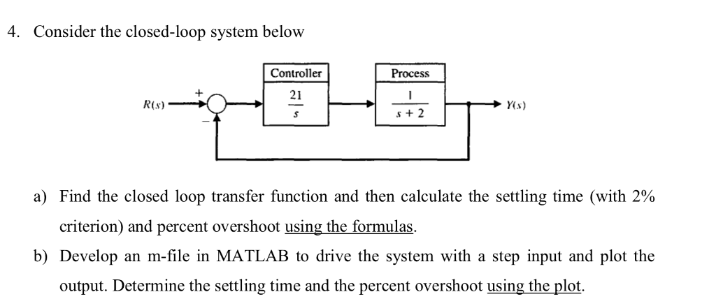
Solved A Find The Closed Loop Transfer Function And Then Chegg Com

Control Tutorials For Matlab And Simulink Motor Position Digital Controller Design
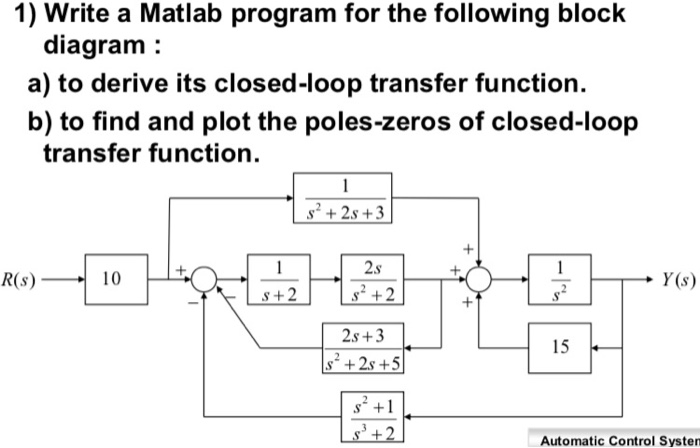
Solved 1 Write A Matlab Program For The Following Block Chegg Com

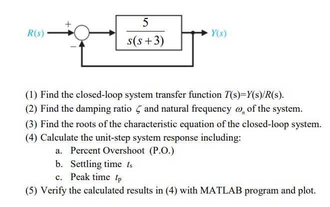
Solved R S Y S 1 Find The Closed Loop System Transfer Chegg Com
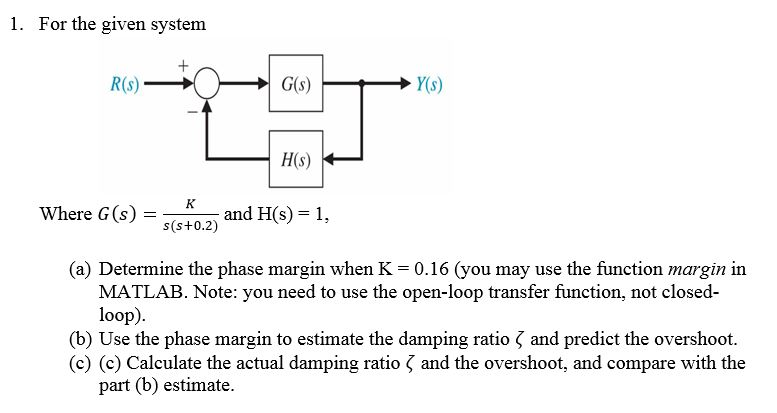
Solved For The Given System Determine The Phase Margin Wh Chegg Com

Use Of Matlab 3 Closed Loop Transfer Functions Youtube
In Matlab Use A For Loop To Evaluate The System F Chegg Com

Matlab Simulink Closed Loop Transfer Function Block Diagram Download Scientific Diagram
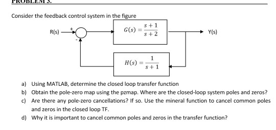
Solved Consider The Feedback Control System In The Figure Chegg Com
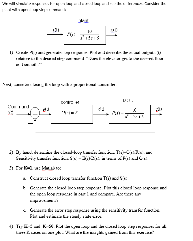
Solved We Will Simulate Responses For Open Loop And Close Chegg Com
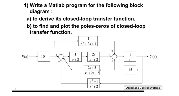
Solved 1 Write A Matlab Program For The Following Block Chegg Com
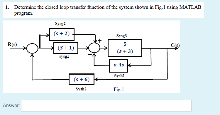
Solved 1 Determine The Closed Loop Transfer Function Of Chegg Com

Solved 1 For The Unity Feedback Control System Shown Her Chegg Com
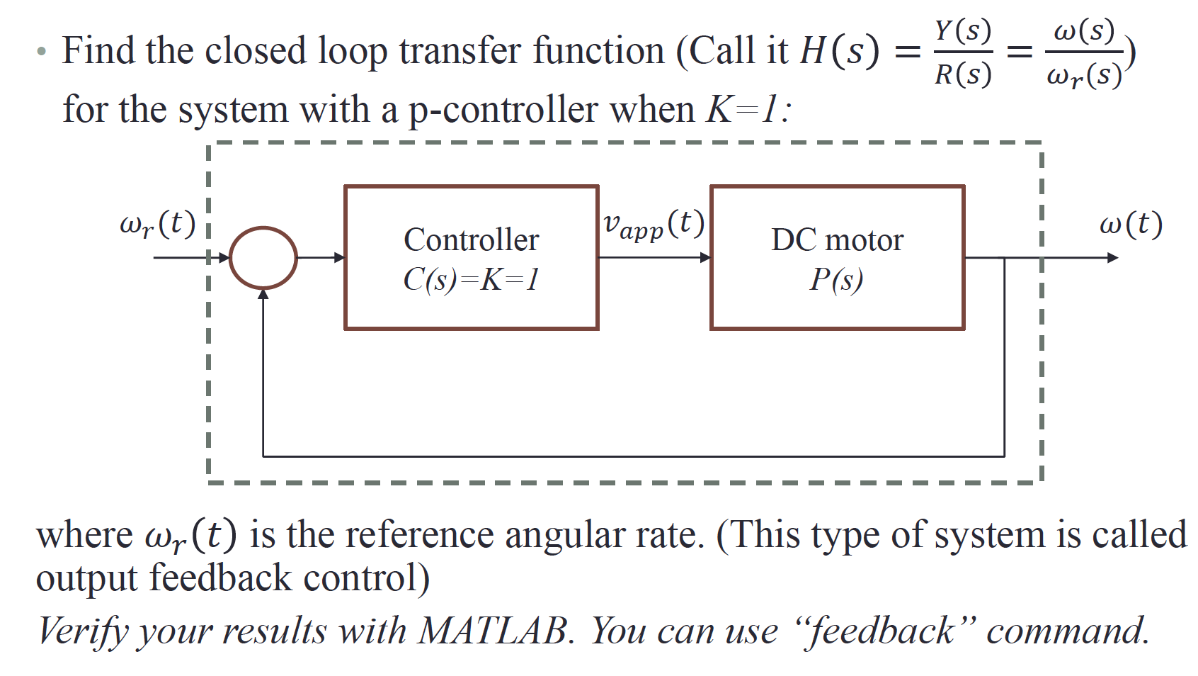
Solved Find The Closed Loop Transfer Function Call It Chegg Com
Solved Task Create Transfer Functions In Two Different M Chegg Com
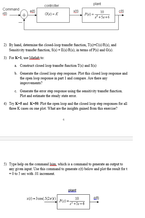
Solved Plant Controller Command R T P S 2 By Hand Det Chegg Com
Https Encrypted Tbn0 Gstatic Com Images Q Tbn 3aand9gcrkhcovzptfzrysveci Jkaywyau84aozccy3s8m6u8g U8fgxr Usqp Cau
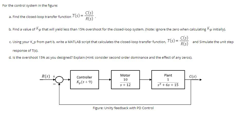
Solved For The Control System In The Figure A Find The Chegg Com

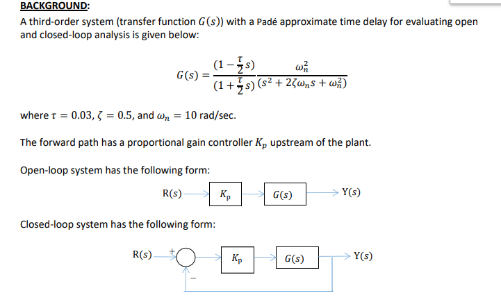
Problem 4 Consider The Control System Shown Below With Plant G S That Has Time Con Stants Homeworklib
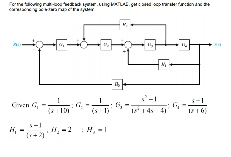
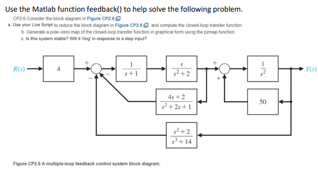
Solved For The Following Multi Loop Feedback System Usin Chegg Com
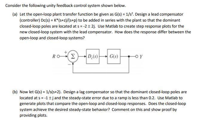
Solved Consider The Following Unity Feedback Control Syst Chegg Com
1 Find The Compensator Open Loop Transfer Functio Chegg Com
Source : pinterest.com
